Introduction to Bayesian inference with PyStan – Part II

This is the continutation of the first part of the blog post on this topic. If you are completely new to the topic of Bayesian inference, please don’t forget to start with the first part, which introduced Bayes’ Theorem.

This second part focuses on examples of applying Bayes’ Theorem to data-analytical problems.

A simple example

Imagine, we want to estimate the fairness of a coin by assessing a number of coin tosses. The parameter we want to estimate is in this case the probability that a coin falls (assuming that the tossing-process is unbiased) on its head.

$\theta$

Obviously, a fair coin would be characterized by

$\theta = 0.5$

The (binomial) Likelihood

The data we observe consists of a a number of “Heads” and “Tails”. Let’s assume we have N_H heads out of N coin tosses. In this case (assuming that all coin tosses are independent of each other and identically distributed (i.i.d.)), the probability of the data given the parameter is given by a binomial likelihood:

$p(N_H | \theta) = \binom{N}{N_H} \theta^{N_H} \left(1-\theta\right)^{N-N_H}$

The prior distribution

In order to have a fully specified Bayesian model, we need to specify a prior distribution over all parameters of the model. In this case, we have only one free parameter: theta. The conventional choice in this case is a beta distribution. The beta distribution is defined for input values from 0 to 1 – thus suitable for a probability parameter. Another reason for choosing the Beta distribution is the fact, that it is a conjugate distribution for the binomial likelihood – which will make calculations easier.

Choosing a conjugate distribution as a prior distribution will lead to a posterior distribution which has the same form as the prior distribution. The conjugate prior distribution for a binomial likelihood is the beta distribution [1]:

$p\left(\theta\right) = \frac{\theta ^{\alpha -1} \left(1-\theta\right)^{\beta-1}}{B\left(\alpha,\beta\right)}$

The normalization constant B is the so-called Beta function.

The posterior distribution

Using Bayes’ Theorem, we obtain the following expression for calculating the posterior distribution:

$p(\theta|N_H) = \frac{p(N_H|\theta) p(\theta)}{\int_{0}^{1} p(N_H|\theta^{*})p(\theta^{*})d\theta^{*}}$

If we plug in the prior and the likelihood and ignore all normalizing constants, we obtain:

$p(\theta|N_H) \propto \theta^{\alpha + N_H – 1} \left(1-\theta \right)^{\beta + N – N_H – 1}$

The posterior distribution thus follows exactly the same form as the prior distribution – which was one of the reasons we chose the Beta distribution in the first place. We know

• a) that the posterior distribution is normalized
• b) that the posterior distribution is a Beta distribution
• c) the normalizing factor for a Beta distribution (Beta function in the denominator)

Thus, the posterior is given by:

$p\left(\theta\right) = \frac{\theta ^{\alpha’ -1} \left(1-\theta\right)^{\beta’-1}}{B\left(\alpha’,\beta’\right)}$

with:

$\alpha’ = \alpha + N_H$
$\beta’ = \beta + (N – N_H)$

Going from the prior to the posterior in this case simply implies to update the parameters of the Beta distribution. The initial parameter alpha is updated by adding the number of “positive” observations (number of heads). The parameter beta is updated by adding the number of “negative” observations (total coin tosses minus the number of heads).

This leads to the following interpretation: The parameter alpha in the prior distribution can be regarded as the number of initial positive observations minus one. The parameter beta in the prior distribution can be interpreted as the initial number of negative (tails) observations minus one.

Upon observation of actual data, the parameters get updated accordingly (the number of positive observations gets added to alpha, the number of “tail” – observations gets added to beta).

The Beta distribution is identical to the continuous uniform distribution on the interval [0,1] for values alpha=1 and beta = 1. This is identical to 0 prior observations of “heads” and 0 prior observations of “tails”.

 

Plotting the prior, the posterior and the Likelihood

Let’s look at a visualization of prior distribution, likelihood function and posterior distribution for this case:

I have chosen a prior distribution with parameters alpha=2 and beta=2. As a reminder: This can be interpreted as corresponding to the prior observation of 1 “heads” and 1 “tails”. It is therefore symmetric around 0.5 and has a probability density of 0 at the values for theta of 0 and 1.0. This of course makes sense – after all 1 “head” has already been observed, so the probability of heads can not be 0 anymore. The same goes for the probability of “heads only” (at theta=1.0). This has to be 0 because 1 “tail” has already been observed.

The likelihood function is plotted for the value of N=3 total coin tosses, out of which all – N_heads=3 – turned out “heads”. The value of the likelihood function at theta=0 is again zero – reflecting the fact that it’s impossible to observe 3 “heads” if the underlying probability for “heads” is zero. The highest likelihood is given for a value of theta=1.0 – reflecting the fact that the value of theta that makes the observation of 3 heads in 3 coin tosses the most probable is 1.0. As a further note: The likelihood function is not a (normalized) probability distribution as are the prior and the posterior distribution – so don’t be surprised if “integrating the curve in your head” doesn’t result in a value of 1 for the area.

The posterior distribution is the product of the prior distribution and the likelihood function. It is in a sense a compromise between both. The prior distribution had its probability mass spread out symmetrically around the value 0.5. Due to the observation of 3 “heads” in 3 coin tosses, the posterior distribution has its probability mass strongly shifted to higher values. Typically – as it is also the case here – the posterior distribution is significantly more narrow than the prior distribution. The reason is simple: It is based on the observation of additional data and thus is “more certain”.

There are multiple ways of reporting the result of a Bayesian analysis. The three black points in the posterior distribution show (from left to right) the mean, the median and the mode of the posterior distribution. It certainly doesn’t hurt to report one or more of these point estimates. Yet, it should be mentioned that the spirit of Bayesian data analysis is exactly not to rely too strongly on point estimates. Neither of the aforementioned point estimates (median, mean or mode) provide the full picture. The entire information is incorporated in the distribution.

Another way of reporting results of a Bayesian data analysis is by communicating the boundaries of Credible Intervals. These are the Bayesian equivalent of Confidence Intervals. Confidence intervals are often misinterpreted as Bayesian Credible intervals. A 80% credible interval contains with a probability of 80% the true value of a parameter. There are different ways of constructing a credible interval. Depicted in the figure above is a credible interval from the 10th to the 90th percentile of the posterior distribution (area filled in blue). The area under the posterior curve to the left of the area filled in blue is identical to the area to the right of the interval. The area filled in red is the so-called highest density interval (HDI). It also contains 80% of the probability density, but is the narrowest range that does so.

 

Inference with (Py)Stan

We obtained the posterior distribution in this case analytically – making use of the “cheap” trick of a conjugate prior. So, we have no actual need of using Pystan in this case. But to demonstrate the functionality of Pystan we will do it anyways 😉 .

The program Stan has its own modelling language. Model specifications in Stan are usually saved in a *.stan – file. It contains several sections – the input data is specified in the data – section, the parameters are specified in the parameters section and the model (likelihood function and prior distributions) are specified in the model section. There exist more sections that provide for example the functionality to specify user defined functions or the possibility to directly generate simulations based on the inferred parameters . We don’t necessarily need these additional sections here.

/model/bin_lik_beta_prior.stan: (code can be found in the GitHub – repository) : https://github.com/DataInsightsGmbH/pystan_examples

data {
  int<lower=0>N_heads;
  int<lower=0>N_tails; 
}

parameters 
{
  real<lower=0,upper=1> theta;
}
model 
{
  theta ~ beta(2, 2);
  N_heads ~ binomial(N_heads + N_tails, theta);
}

// alternate model specification (commented out here)
// might be more intuitive: directly specifies the increments of the 
// log posterior density, i.e. the log posterior density apart from an 
// additive constant
//model
//{
//  target+=beta_lpdf(theta|2,2);
//  target+=binomial_lpmf(N_heads|N_heads+N_tails,theta);
//}

 

The data section in the above listing tells Stan the names (N_heads, N_tails), types (integers) and potentially constraints (here: positivity) of the data.

If you call Stan via PyStan from Python, then you can pass the data in a dictionary, where the names of the keys have to be identical to the names specified in the *.stan – model file.

The parameters – section tells Stan the names, types and constraints of the parameters. In this case, we call the probability of heads theta and define it to be a real valued (continuous) parameter between 0 and 1.

The model – section serves to specify the posterior distribution. The syntax might need some getting used to. The first line specifies the prior distribution for the parameter theta. It’s a beta distribution with (hyper)parameters alpha=2 and beta=2. The second line specifies the likelihood function – a binomial distribution with probability for heads theta, total number of observations N_heads + N_tails and N_heads actual observations of “heads”.

The posterior distribution can be specified in a slightly different – and maybe easier to read – way. In order to motivate it, let’s take the logarithm of the posterior distribution:
$\text{log} \, p\left(\theta|N_H\right) = \text{log} \, p\left(N_H|\theta\right) + \text{log} \, p \left(\theta\right) – \text{log} \left[ \int_{0}^{1} p(N_H|\theta^{*})p(\theta^{*})d\theta^{*}\right]$
The last term (the marginal likelihood) does not depend on the parameter theta (it’s integrated out). It can therefore be regarded as a constant. We can thus write:

$\text{log} \, p\left(\theta|N_H\right) = \text{log} \, p\left(N_H|\theta\right) + \text{log} \, p \left(\theta\right) + C$

Meaning the logarithm of the posterior distribution is given by the sum of the logarithms of the likelihood function and the prior. In Stan – Code this is specified in the following way:

....
model
{
  target+=beta_lpdf(theta|2,2);                           // add the logarithm of the beta pdf to the log posterior
  target+=binomial_lpmf(N_heads|N_heads+N_tails,theta);   // add the logarithm of the binomial pmf to the log posterior
}

Again, both ways result in the specification of the same model. Yet, I would imagine that the second version is probably more intuitive for people who haven’t worked with Stan or similar software before.

What remains to be done is:

1. load the model (into a string)

2. compile the model

3. pass data

4. let Stan create samples for us

The code for doing this is shown in the listing below:

conduct_inference.py: (excerpt)

#.....

PATH_STAN_MODELS = 'models'                # <-- path for the *.stan (stan models) files
FN_BLBP_MODEL = 'bin_lik_beta_prior.stan'  # <-- definition of our model (prior, likelihood)

if __name__=='__main__':
    data_for_stan = {'N_heads':3,
                     'N_tails':0}          # <-- prepare the "data" that will be handed over to Stan
                                           # keys in this dictionary need to have the same names as the 
                                           # variables in the *.stan - file
                                           
# load the model code into a string:
    comp_path_stan_model = os.path.join(PATH_STAN_MODELS,FN_BLBP_MODEL)
    with open(comp_path_stan_model,'rt') as sm_file:
        model_code_str = sm_file.read()
    # compile the model (this may take several minutes):
    stan_model =  pystan.StanModel(model_code=model_code_str)
    stan_fit   = stan_model.sampling(data=data_for_stan,
                             iter=20000,
                             chains=1
                            )

 

We first open the file and read the file’s contents (the complete model specification) into a string.

Afterwards, pystan.stanModel is called with the model (string) as a parameter. Stan will subsequently compile the model (into C++ – code). This usually can take up to a couple of minutes.

The object that was returned from the pystan.stanModel – function has a method called sampling that can to actually create samples. The data should be passed as a Python dictionary. Additionally, the number of iterations and the number of chains (for simplicity’s sake here 1) can be specified. The usage of multiple chains (=sequences of samples) is usually recommended because significant differences in the statistics of samples from different chains can be indicative of problems with the sampling.

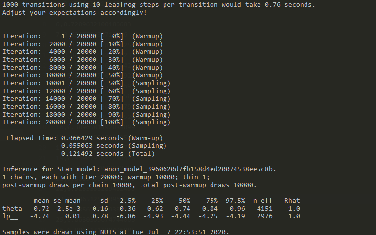
The duration of the sampling can vary strongly with model complexity and number of samples. Here, the generation of 20 000 samples (the first 10 000 of which will be discarded) took around 0.12s. Obviously, the inference of more complex models can take significantly longer. In general, one should take as many samples as possible (constraint usually by computational resources / time). The more samples we obtain, the more precisely any statistic we would like to obtains (mean, stdev,….) can be estimated from the samples.

Let’s take another look at Stan’s output above: It tells us that there have been 20 000 samples generated, the first 10k were ignored (warmup = 10000) and every sample afterwards is retained (thin=1). In addition, Stan provides us with summary statistics about the inferred parameter and the value of the log posterior (up to some constant). For example, the mean, the standard error of the mean, the standard deviation and a number of quantiles are provided for the parameter and the log posterior. In addition, the number of effective samples n_eff are specified.

Samples that Stan creates are correlated and thus the number of “effective” / independent samples is usually smaller than the number of samples (here: n_eff = 4151, number of samples =10000). This correlation of samples is typical for MCMC methods in general (it doesn’t create independent samples) – but usually not too problematic if the effective sample size is still “high” (in the thousands). That is another convergence diagnostic. Values significantly above 1.0 are a cause for concern.

So, now that Stan did the sampling for us, we somehow have to make them accessible from within Python:

stan_fit   = stan_model.sampling(data=data_for_stan,
                             iter=2*NUM_SAMPLES,
                             chains=1
                            )
thetas = np.array(stan_fit["theta"])

Afterwards, we can simply work with the numpy array (or Python list if we prefer) as desired.

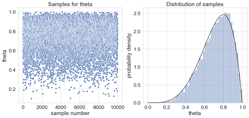
The following graph illustrates “the magic”: We plotted the 10 000 samples in the left panel. The right panel shows the distribution of the samples – super-imposed as a black line is a beta distribution with parameters alpha=5 and beta = 2 (the posterior distribution we calculated for N_heads = 3, N_tails = 0 and a beta prior with alpha=2 and beta=2).

So, that’s exactly what sampling with Stan is about: We specify a likelihood function and a prior over all parameters and obtain samples which are distributed according to the posterior distribution.

 

Bayesian Logistic Regression

 

Let’s look at an example with a little bit more “real-world” appeal. Let’s assume that we have data of a number of students: We know how long they studied for a particular exam and whether they passed or not (this example is borrowed from the Wikipedia page for “Logistic Regression” – we will use it to illustrate the Bayesian way of “fitting” a Logistic Regression model).

We will first simulate some data according to a logistic regression model and subsequently use Stan to do the inference for us.

Logistic regression is a member of a class of statistical models called Generalized Linear Models.

A linear predictor function is mapped to the interval between 0 and 1 (we are dealing with probabilities) by being transformed by a logistic function. The outcome variable is assumed to be Bernoulli – distributed (being either 0 or 1, the underlying probability is given by the transformed linear predictor).

Let’s first use Python to simulate some test data. We first sample the preparation times for the exam from a continuous uniform distribution (minimum 1.0 hour, maximum 12.0 hours). The probability for passing is subsequently calculated by:

1. linearly transforming the “hours” (a*x+b) – students that studied longer are supposed to increase their chances of passing the exam

2. applying a logistic function to map the results of the linear transform to values from 0 to 1

3. the outcome “passed” is finally obtained by sampling from a Bernoulli distribution (binomial with n=1)

The code for creating test data is shown below:

import numpy as np
def logistic_function(x,a,b):
  return 1.0/(1.0 + np.exp(-(a*x+b)))
a=0.6;b=-4.0;num_samples=15
num_samples = 15
hours = np.random.uniform(low=1.0,high=12.0,size=num_samples)
probs = [logistic_function(hour,a=a,b=b) for hour in hours]
passed = [np.random.binomial(n=1,p=p_i,size=1)[0] for p_i in probs]

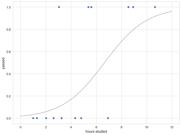
The simulated test data (here for 15 students) as well as the underlying (studying-time depended) probability for passing is shown in the figure below:

The Stan model for doing inference on this model is given below. We pass the total number of data points N (the number of students) and for each student the number of hours they studied as well as whether they passed. In this case, we have two parameters (for the linear predictor, the intercept beta and the slope alpha).

In this case we haven’t specified prior distributions on the parameters. This implicitly makes the parameters have uniform distributions. In this case, the MAP of the posterior distribution will be almost (apart from numerical issues / sampling error) identical to the Maximum Likelihood Estimate.

The specification of the likelihood might again need some getting used to. Basically all the transformations (logistic function as well as Bernoulli distribution) are packed into one line 😉 :

Stan – Model for Logistic Regression with one predictor (see e.g. Stan-Manual):

data {
  int<lower=0> N;
  vector[N] hours;
  int<lower=0,upper=1> passed[N];
}
parameters {
  real alpha;
  real beta;
}
model {
  passed ~ bernoulli_logit(alpha * hours + beta);
}

The code for compiling the model and sampling from it is very similar to the code from the first example.

We again call the StanModel function and the sampling method:

NUM_SAMPLES = 10000
PATH_STAN_MODELS = 'models'
FN_LR_MODEL = 'logistic_regression.stan'

data_for_stan = {"N":NUM_DATA_POINTS,"x":hours,"y":passed}
comp_path_stan_model = os.path.join(PATH_STAN_MODELS,FN_LR_MODEL)

with open(comp_path_stan_model,'rt') as sm_file:
  model_code_str = sm_file.read()

stan_model =  pystan.StanModel(model_code=model_code_str)
stan_fit   = stan_model.sampling(data=data_for_stan,
                                 iter=2*NUM_SAMPLES,
                                 chains=1
                                )
df_stan_samples = pd.DataFrame({"alpha":list(stan_fit["alpha"]),"beta":list(stan_fit["beta"])})

As already mentioned, we obtain samples for two different parameters this time (slope and intercept for each linear predictor). The samples of these parameters are displayed in the left panel below. We can see a couple of thousand samples for the parameters alpha (x-axis) and beta (y-axis). Each pair of parameters describes a logistic curve. To illustrate this further, 4 points have been picked (basically at random). The corresponding 4 logistic curves (calculated by plugging in the value for alpha and beta for that sample) are shown in the panel in the middle.

Samples are distributed according to the posterior distribution ( somewhat centered around alpha=0.6 .. 0.7 and beta = -4.0 .. -4.5). Each sample corresponds to one logistic curve. The distribution of the points determines also the distribution of the logistic curves. We can calculate the “mean curve” (black line) and the 80% credible interval (blue region) for the logistic curve – giving us an estimate of the curve as well as the curve’s uncertainty.